Marital correlations
Social Diagnosis is a series of studies that concluded nearly a decade ago, yet the publicly available survey data still allow us to uncover interesting relationships and patterns. One such example is the correlation between spouses. Let’s examine how husbands and wives correlate in terms of age, height, weight, and income.
The survey data can be found on GitHub, where Prof. Przemysław Biecek has prepared files that can be directly loaded into R. The following command loads the data frame named osoby (“individuals”):
load(url("https://github.com/pbiecek/Diagnoza/raw/master/data/osoby.rda"))
From the dataset, we select only the variables we need: identifiers, gender, age, height, weight, income, and survey weights. According to Prof. Biecek’s documentation, variables from the year 2015 start with the letter h.
extract <- osoby[, c('numer_gd', 'numer_osoby', 'hc5', 'hc6', 'hc10',
                     'hp65', 'hp52', 'hp53', 'waga_2015_ind', 'wiek2015')]
names(extract) <- c('household_id', 'person_id', 'family_no', 'family_role',
                    'sex', 'income', 'height', 'weight', 'survey_weight', 'age')
Since the original data frame covers all years of the study, many records contain missing values (NA). After several trials and data inspections, I found the following approach most effective: temporarily replace NA in the income column with -1 (to avoid removing observations with missing income, such as retirees), then remove rows with other missing values, and finally restore NA in the income variable.
extract$income[is.na(extract$income)] <- -1
extract <- na.omit(extract)
extract$income[extract$income == -1] <- NA
Next, we create a family identifier (family_id) to link husband and wife data.
extract$family_id <- paste(extract$household_id, extract$family_no)
We then select husbands and wives separately:
extract_husband <- extract[(extract$family_role == 1 | extract$family_role == 2) &  extract$sex == 1,
                           c('family_id', 'income', 'height', 'weight', 'survey_weight', 'age')]
names(extract_husband) <- c('family_id', 'husband_income', 'husband_height', 'husband_weight',
                            'husband_survey_weight', 'husband_age')

extract_wife <- extract[(extract$family_role == 1 | extract$family_role == 2) & extract$sex == 2,
                        c('family_id', 'income', 'height', 'weight', 'survey_weight', 'age')]
names(extract_wife) <- c('family_id', 'wife_income', 'wife_height', 'wife_weight',
                         'wife_survey_weight', 'wife_age')
After merging the husband and wife data, we obtain the data frame e, where each row corresponds to one couple.
e <- merge(extract_husband, extract_wife)
The study authors provided survey weights, which allow us to adjust the results to account for the fact that not every person had an equal chance of being included in the sample. I assume that the weight for a couple is the average of the husband’s and wife’s weights. I then scale the weights so that their sum equals the number of couples in the sample.
e$avg_survey_weight <- (e$husband_survey_weight + e$wife_survey_weight)/2
e$avg_survey_weight <- e$avg_survey_weight / mean(e$avg_survey_weight)
head(e)
##   family_id husband_income husband_height husband_weight husband_survey_weight
## 1  100004 1           4000            176             79             0.5515697
## 2  100009 1           2400            182             90             0.5929627
## 3  100014 2           2800            181            120             1.4742120
## 4  100015 1           1800            170             87             0.9607670
## 5  100018 1           3000            175             82             0.7655140
## 6  100021 1           1400            185             92             0.3082680
##   husband_age wife_income wife_height wife_weight wife_survey_weight wife_age
## 1          66        1000         157          51          0.4846472       58
## 2          42        1400         168          57          0.6888809       39
## 3          43        1000         172          80          1.4206220       45
## 4          64        1300         160          68          0.8562090       62
## 5          47        2000         159          75          0.7330340       45
## 6          47        1000         170         104          0.2951890       47
##   avg_survey_weight
## 1         0.5390513
## 2         0.6668290
## 3         1.5059241
## 4         0.9452107
## 5         0.7795610
## 6         0.3139249
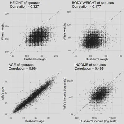
Let’s examine four dimensions of similarity between couples:
-
height,
-
weight,
-
age,
-
income.
For each, we calculate the Pearson correlation coefficient, taking survey weights into account.
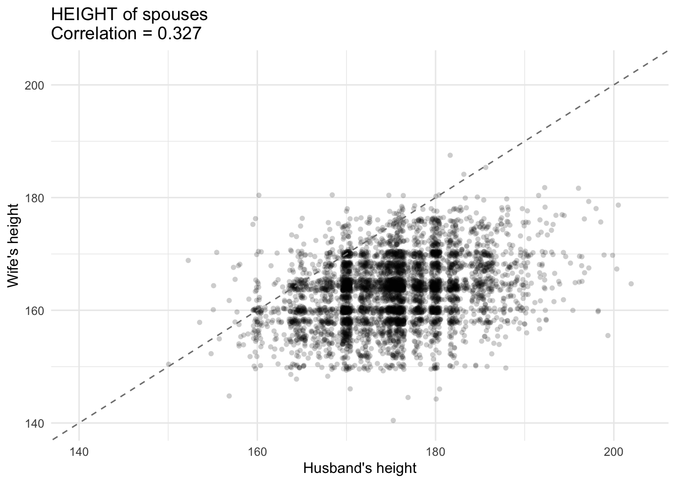
cor_height <- cov.wt(data.frame(e$husband_height, e$wife_height),
                     wt = e$avg_survey_weight, cor = TRUE)$cor[2,1]

library(ggplot2)

min_val <- min(e$husband_height, e$wife_height, na.rm = TRUE)
max_val <- max(e$husband_height, e$wife_height, na.rm = TRUE)

G1 <- ggplot(e, aes(x = husband_height, y = wife_height)) +
  geom_jitter(alpha = 0.2, width = .5, height = .5, shape = 16) +
  geom_abline(intercept = 0, slope = 1, linetype = "dashed", color = "grey50") +
  scale_x_continuous(limits = c(min_val, max_val)) +
  scale_y_continuous(limits = c(min_val, max_val)) +
  labs(
    x = "Husband's height",
    y = "Wife's height",
    title = paste0("HEIGHT of spouses \n", "Correlation = ", round(cor_height, 3))
    ) +
  theme_minimal()
G1
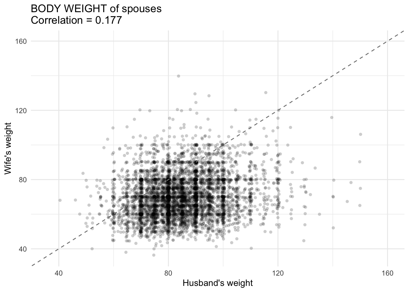
cor_weight <- cov.wt(data.frame(e$husband_weight, e$wife_weight),
                     wt = e$avg_survey_weight, cor = TRUE)$cor[2,1]

library(ggplot2)

min_val <- min(e$husband_weight, e$wife_weight, na.rm = TRUE)
max_val <- max(e$husband_weight, e$wife_weight, na.rm = TRUE)

G2 <- ggplot(e, aes(x = husband_weight, y = wife_weight)) +
  geom_jitter(alpha = 0.2, width = .5, height = .5, shape = 16) +
  geom_abline(intercept = 0, slope = 1, linetype = "dashed", color = "grey50") +
  scale_x_continuous(limits = c(min_val, max_val)) +
  scale_y_continuous(limits = c(min_val, max_val)) +
  labs(
    x = "Husband's weight",
    y = "Wife's weight",
    title = paste0("BODY WEIGHT of spouses \n", "Correlation = ", round(cor_weight, 3))
    ) +
  theme_minimal()
G2
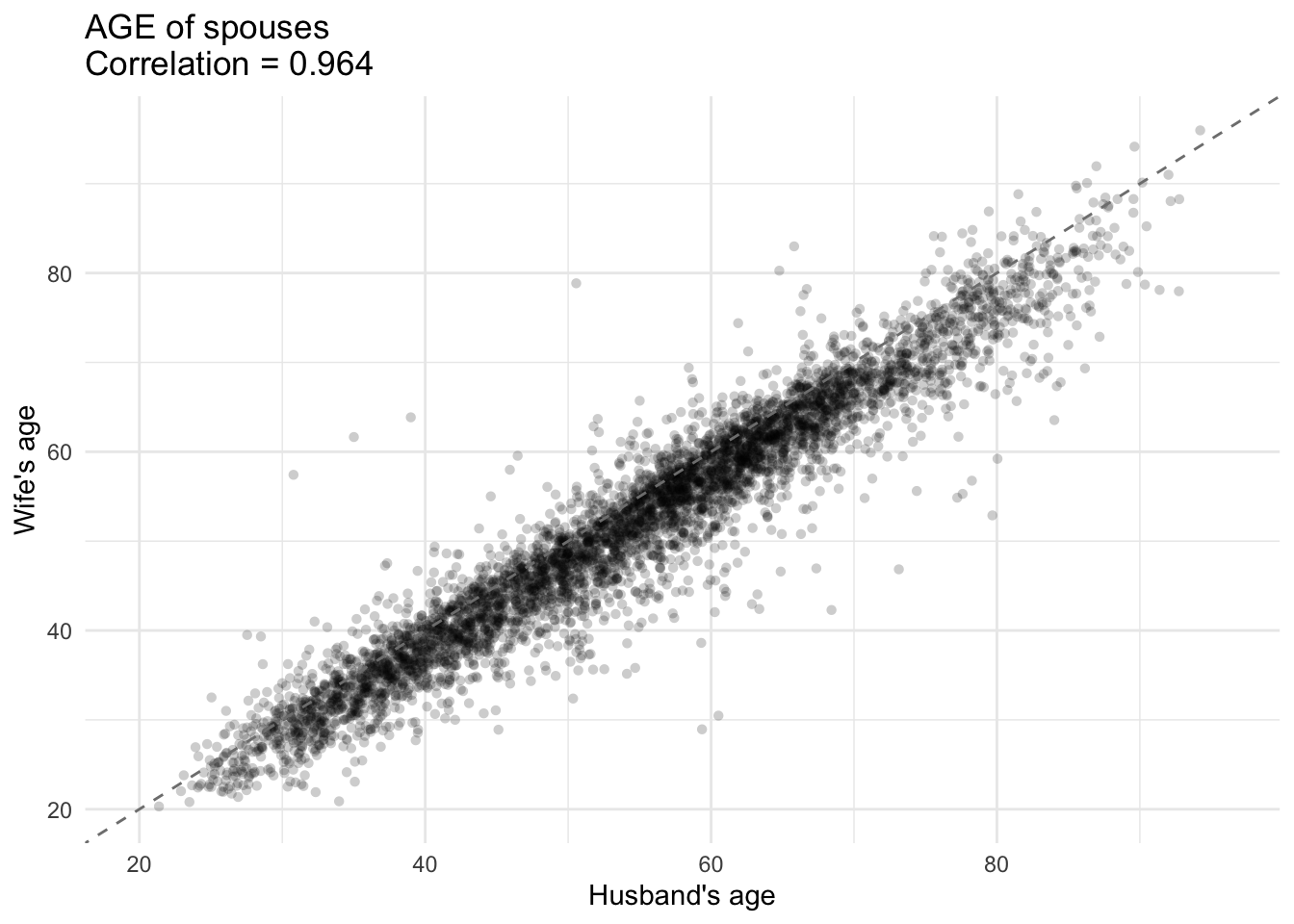
cor_age <- cov.wt(data.frame(e$husband_age, e$wife_age),
                     wt = e$avg_survey_weight, cor = TRUE)$cor[2,1]

library(ggplot2)

min_val <- min(e$husband_age, e$wife_age, na.rm = TRUE)
max_val <- max(e$husband_age, e$wife_age, na.rm = TRUE)

G3 <- ggplot(e, aes(x = husband_age, y = wife_age)) +
  geom_jitter(alpha = 0.2, width = .5, height = .5, shape = 16) +
  geom_abline(intercept = 0, slope = 1, linetype = "dashed", color = "grey50") +
  scale_x_continuous(limits = c(min_val, max_val)) +
  scale_y_continuous(limits = c(min_val, max_val)) +
  labs(
    x = "Husband's age",
    y = "Wife's age",
    title = paste0("AGE of spouses \n", "Correlation = ", round(cor_age, 3))
    ) +
  theme_minimal()
G3
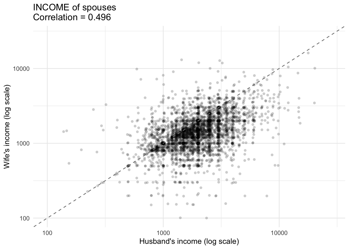
e2 <- na.omit(e[, c('husband_income', 'wife_income', 'avg_survey_weight')])

cor_income <- cov.wt(data.frame(e2$husband_income, e2$wife_income),
                     wt = e2$avg_survey_weight, cor = TRUE)$cor[2,1]

library(ggplot2)

min_val <- min(e2$husband_income, e2$wife_income, na.rm = TRUE)
max_val <- max(e2$husband_income, e2$wife_income, na.rm = TRUE)

G4 <- ggplot(e2, aes(x = husband_income, y = wife_income)) +
  geom_jitter(alpha = 0.2, width = .01, height = .01, shape = 16) +
  geom_abline(intercept = 0, slope = 1, linetype = "dashed", color = "grey50") +
  scale_x_log10(limits = c(min_val, max_val)) +
  scale_y_log10(limits = c(min_val, max_val)) +
  labs(
    x = "Husband's income (log scale)",
    y = "Wife's income (log scale)",
    title = paste0("INCOME of spouses \n", "Correlation = ", round(cor_income, 3))
    ) +
  theme_minimal()
G4