How to weigh a dog using a ruler (in R)
Tomorrow, as part of the Baltic Science Festival, we will once again conduct statistics classes for primary school students entitled “How to weigh a dog using a ruler”. Among the instructors we will have students of Economic Analytics at the Faculty of Management and Economics of Gdańsk Tech Great thanks to Przemysław Biecek for the materials!
The first task faced by workshop participants is to estimate the weight of the dog based on its size – see the extract from the comic book prepared a few years ago by prof. Przemysław Biecek.
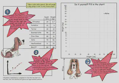
Kids will not be taught linear regression, they will fit the line “by eye”. However, students after the statistics course should try to do it “by the rules”.
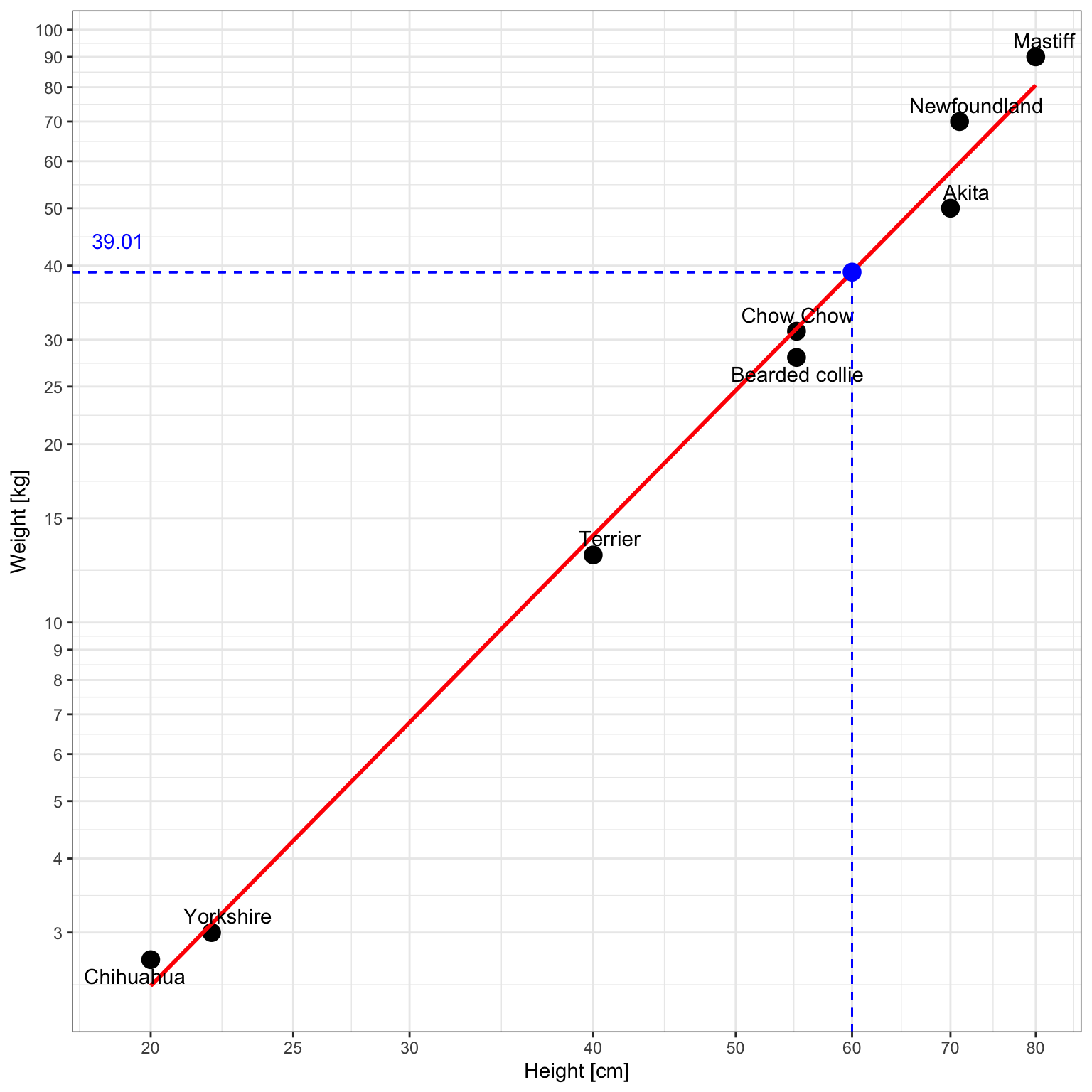
Here’s a graph that predicts the weight of the dog from the comic using simple least squares regression:
Below is a proposed way to do it in R.
Let’s first create a data frame:
size<-c(20, 22, 40, 55, 55, 70, 71, 80)
mass<-c(2.7, 3, 13, 28, 31, 50, 70, 90)
labels<-c("Chihuahua", "Yorkshire", "Terrier", "Bearded collie",
          "Chow Chow", "Akita", "Newfoundland", "Mastiff")
df<-data.frame(size, mass, labels)
df
##   size mass         labels
## 1   20  2.7      Chihuahua
## 2   22  3.0      Yorkshire
## 3   40 13.0        Terrier
## 4   55 28.0 Bearded collie
## 5   55 31.0      Chow Chow
## 6   70 50.0          Akita
## 7   71 70.0   Newfoundland
## 8   80 90.0        Mastiff
Let’s plot the data in a chart:
library(ggplot2)
library(ggrepel)
ggplot(data=df, aes(x=size, y=mass)) +
  geom_point(size=4) +
  xlab("Height [cm]") +
  ylab("Weight [kg]") +
  theme_bw() +
  geom_text_repel(data=df, aes(x=size, y=mass, label=labels))
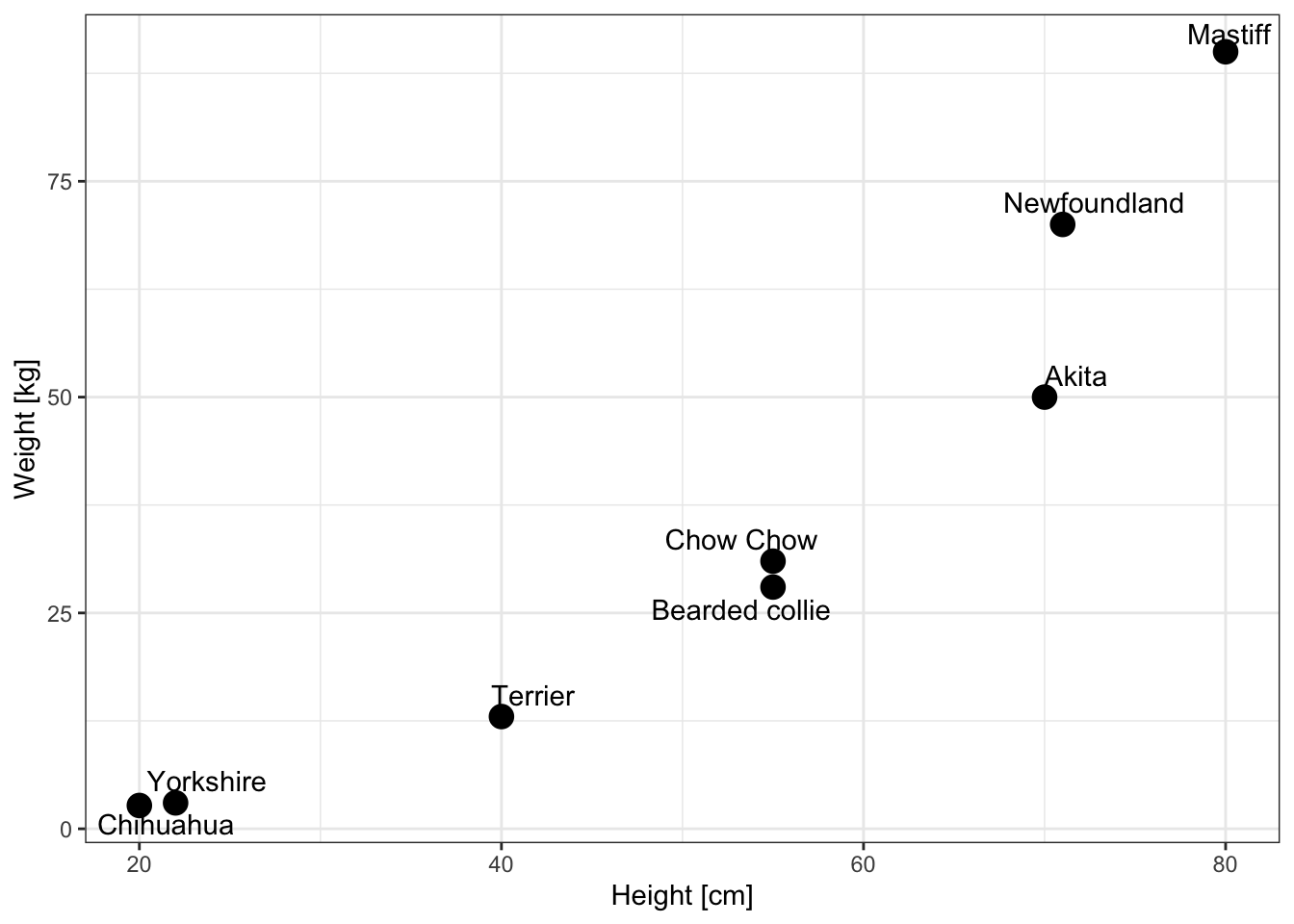
It seems that the relationship between size and mass is not linear. So we will use the power model. In this situation, to use linear regression, both the X and Y variables should be log-transformed.
We won’t disclose it to the kids, but in their comic height and weight are on a log scale (look again at the comic excerpt above). Let’s try to recreate this in R:
yticks<-c(2,3,4,5,6,7,8,9,10,15,20,25,(3:10)*10)
xticks<-c(20, 25, (3:10)*10)

ggplot(df, aes(x=size, y=mass)) +
  geom_point(size=4) +
  xlab("Height [cm]") +
  ylab("Weight [kg]") +
  scale_y_continuous(trans='log10', breaks=yticks) +
  scale_x_continuous(trans='log10', breaks=xticks) +
  theme_bw() +
  geom_text_repel(data=df, aes(x=size, y=mass, label=labels))
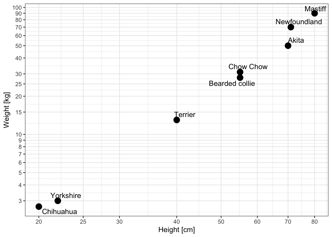
As you can see, it is now possible to draw a straight line approximately matching the points.
Let’s create a power model (linear model on log-transformed variables):
model<-lm(log(mass)~log(size))
summary(model)
##
## Call:
## lm(formula = log(mass) ~ log(size))
##
## Residuals:
##      Min       1Q   Median       3Q      Max
## -0.14068 -0.08472 -0.02180  0.10383  0.16000
##
## Coefficients:
##             Estimate Std. Error t value Pr(>|t|)
## (Intercept)  -6.6678     0.3307  -20.16 9.66e-07 ***
## log(size)     2.5234     0.0855   29.52 1.00e-07 ***
## ---
## Signif. codes:  0 '***' 0.001 '**' 0.01 '*' 0.05 '.' 0.1 ' ' 1
##
## Residual standard error: 0.1207 on 6 degrees of freedom
## Multiple R-squared:  0.9932,	Adjusted R-squared:  0.992
## F-statistic: 871.1 on 1 and 6 DF,  p-value: 1.003e-07
Our model looks like this:
$$\widehat{\text{ln}Y} = -6.6678 + {2.5234} \text{ln}X$$or, equivalently:
$$\widehat{Y} = e^{-6.6678} X ^{2.5234}$$Let’s check (using predict) what the model predicts for a 60-kg dog:
(prediction<-exp(predict.lm(model, newdata=data.frame(size=c(60)))))
##        1
## 39.00646
The model predicts that the dog will weigh approximately 39.01 kg. Mathematically it would look like this:
$$\widehat{Y} = e^{-6.6678} 60 ^{2.5234} \approx 39.01$$Illustration with a ggplot2 chart:
ggplot(df, aes(x=size, y=mass)) +
  geom_point(size=4) +
  xlab("Height [cm]") +
  ylab("Weight [kg]") +
  stat_smooth(method = "lm",
              formula = y ~ x,
              geom = "smooth",
              se=FALSE,
              colour='red') +
  scale_y_continuous(trans='log10', breaks=yticks) +
  scale_x_continuous(trans='log10', breaks=xticks) +
  theme_bw() +
  geom_point(data=data.frame(size=60, mass=prediction, labels="Our Dog"),
             aes(x=size, y=mass),
             colour='blue',
             size=4) +
  geom_text_repel(data=df, aes(x=size, y=mass, label=labels))+
  geom_segment(aes(x=60, y=0, xend=60, yend=prediction), lty=2, col='blue')+
  geom_segment(aes(x=0, y=prediction, xend=60, yend=prediction), lty=2, col='blue') +
  annotate("text", x=min(xticks)-1, y=prediction+5, label=round(prediction,2), col='blue')
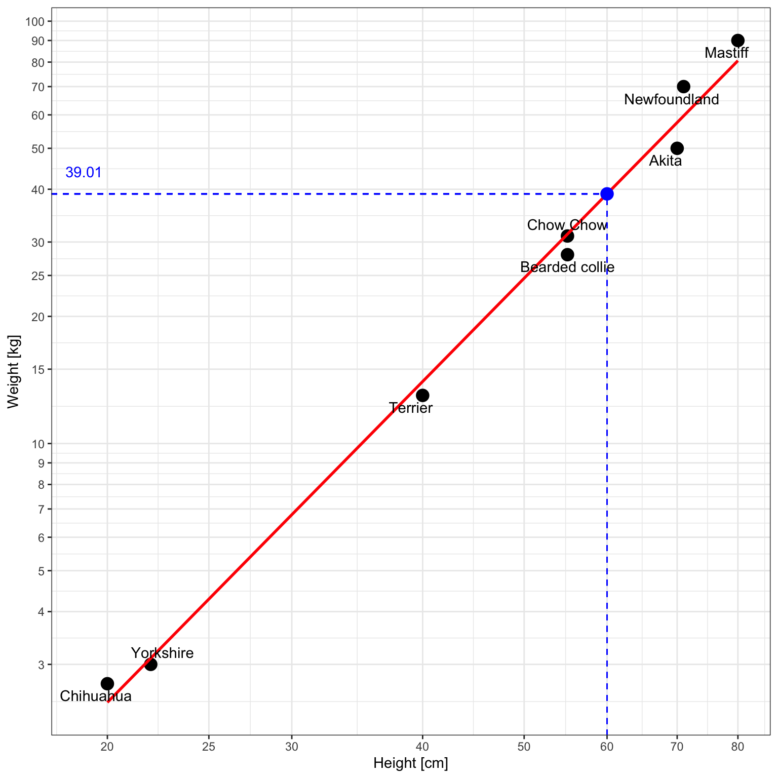
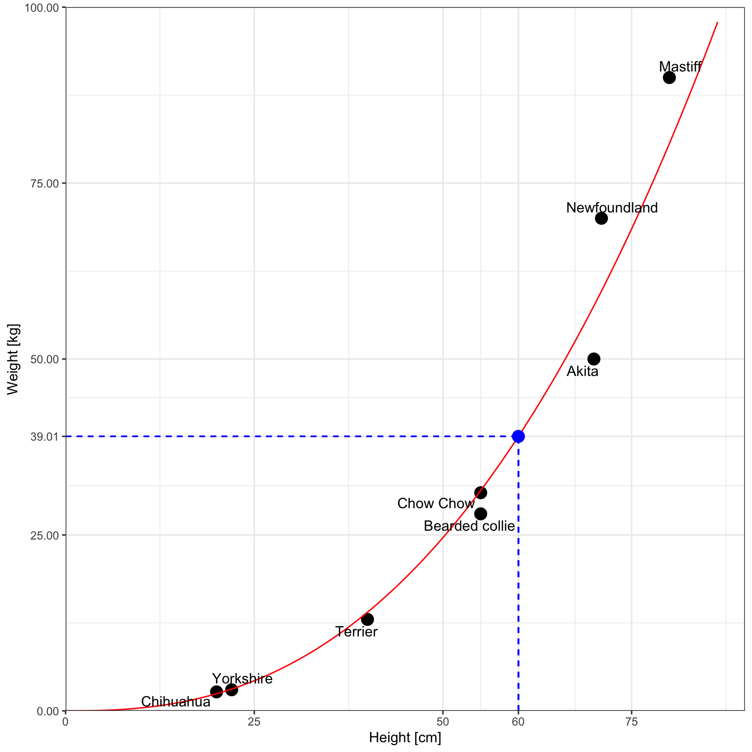
And this is the plot without log-log axes:
ggplot(df, aes(x=size, y=mass)) +
  geom_point(size=4) +
  xlab("Height [cm]") +
  ylab("Weight [kg]") +
  geom_function(fun=function(x){exp(model$coefficients[1])*x^model$coefficients[2]},
                colour='red') +
  scale_x_continuous(limits=c(0,90), breaks=sort(c(0:3*25, 60)), expand = c(0, 0)) +
  scale_y_continuous(limits=c(0,100), breaks=sort(c(0:4*25, as.numeric(round(prediction,2)))), expand = c(0, 0)) +
  theme_bw() +
  geom_point(data=data.frame(size=60, mass=prediction, labels="Our Dog"),
             aes(x=size, y=mass),
             colour='blue',
             size=4) +
  geom_text_repel(data=df, aes(x=size, y=mass, label=labels))+
  geom_segment(aes(x=60, y=0, xend=60, yend=prediction), lty=2, col='blue')+
  geom_segment(aes(x=0, y=prediction, xend=60, yend=prediction), lty=2, col='blue')
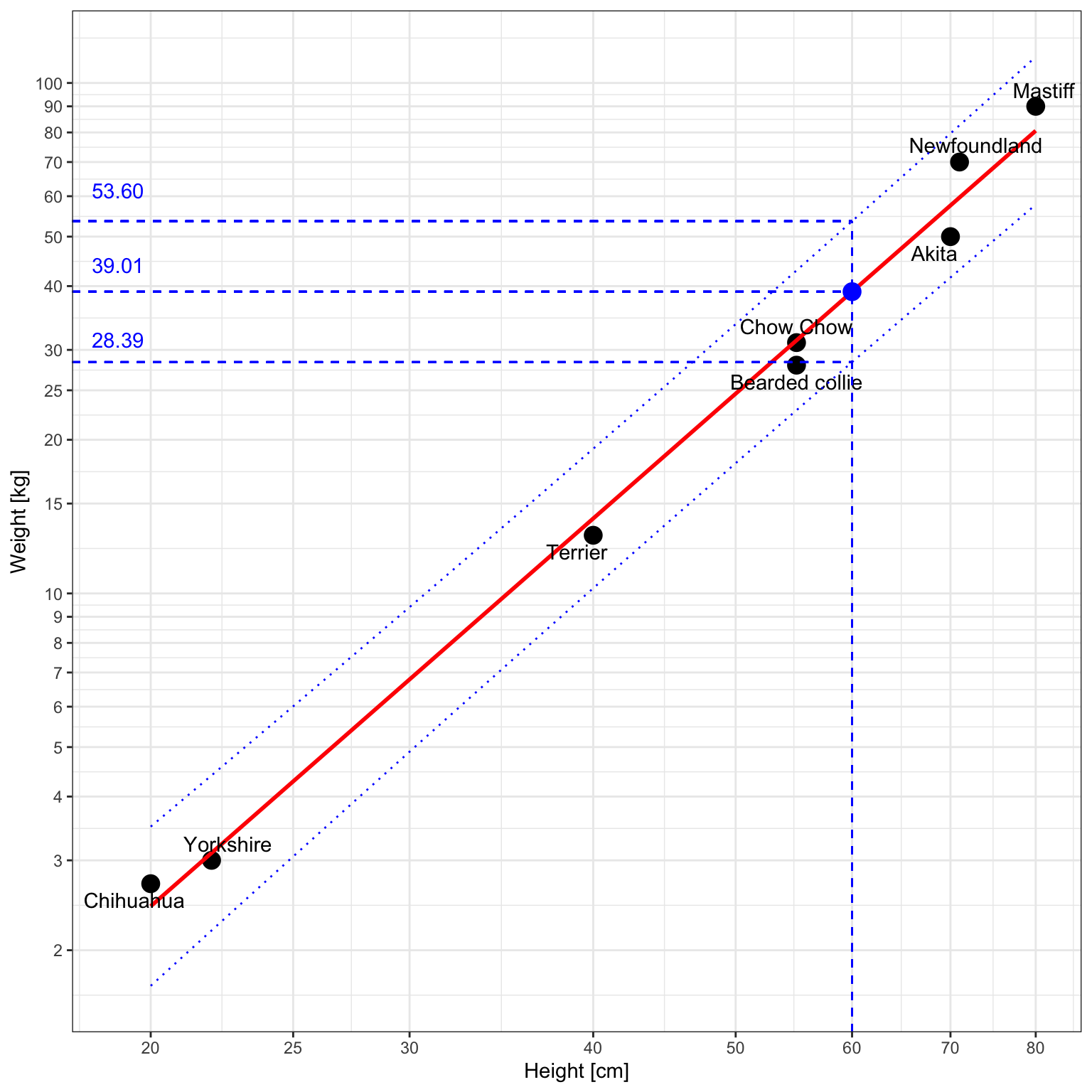
Instead of a point estimate, we can propose an interval estimate. This, of course, requires that the relevant assumptions (the sample is random, the conditional distribution of log(mass) is normal, etc.) are at least approximately met.
The prediction interval for a 60cm dog can be determined as follows:
(prediction_interval<-exp(predict(
  model,
  newdata=data.frame(size=c(60)),
  interval = "prediction",
  level=0.95))
 )
##        fit      lwr      upr
## 1 39.00646 28.38695 53.59872
So, with 95% confidence, we predict that a 60cm dog will weigh between 28.39 a 53.60 kg.
x4pred<-20:80
df3<-data.frame(exp(predict(model, newdata=data.frame(size=x4pred), interval = "prediction", level=0.95)))
df3$x<-x4pred

ggplot(df, aes(x=size, y=mass)) +
  geom_point(size=4) +
  xlab("Height [cm]") +
  ylab("Weight [kg]") +
  stat_smooth(method = "lm",
              formula = y ~ x,
              geom = "smooth",
              se=FALSE,
              colour='red') +
  scale_y_continuous(trans='log10', breaks=yticks) +
  scale_x_continuous(trans='log10', breaks=xticks) +
  theme_bw() +
  geom_point(data=data.frame(size=60, mass=prediction, labels="Nasz Pies"),
             aes(x=size, y=mass),
             colour='blue',
             size=4) +
  geom_text_repel(data=df, aes(x=size, y=mass, label=labels)) +
  geom_segment(aes(x=60, y=0, xend=60, yend=prediction_interval[,3]), lty=2, col='blue') +
  geom_segment(aes(x=0, y=prediction, xend=60, yend=prediction), lty=2, col='blue') +
  annotate("text", x=min(xticks)-1, y=prediction+5, label=format(round(prediction,2), nsmall=2), col='blue') +
  geom_line(data=df3, aes(x=x, y=lwr), col='blue', lty=3) +
  geom_line(data=df3, aes(x=x, y=upr), col='blue', lty=3) +
  geom_segment(aes(x=0, y=lower, xend=60, yend=lower), lty=2, col='blue') +
  annotate("text", x=min(xticks)-1, y=lower+3, label=format(lower, nsmall=2), col='blue') +
  geom_segment(aes(x=0, y=upper, xend=60, yend=upper), lty=2, col='blue') +
  annotate("text", x=min(xticks)-1, y=upper+8, label=format(upper, nsmall=2), col='blue')
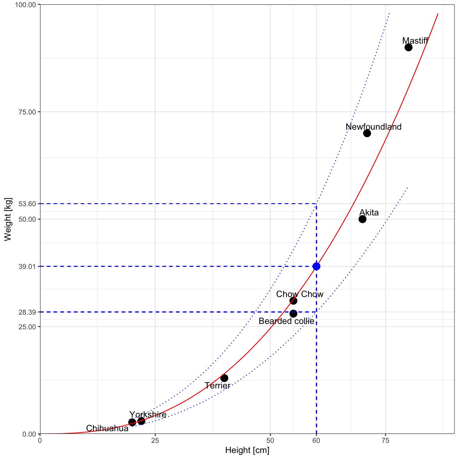
ggplot(df, aes(x=size, y=mass)) +
  geom_point(size=4) +
  xlab("Height [cm]") +
  ylab("Weight [kg]") +
  geom_function(fun=function(x){exp(model$coefficients[1])*x^model$coefficients[2]},
                colour='red') +
  scale_x_continuous(limits=c(0,90), breaks=sort(c(0:3*25, 60)), expand = c(0, 0)) +
  scale_y_continuous(limits=c(0,100), breaks=sort(c(0:4*25, lower, upper, as.numeric(round(prediction,2)))), labels = function(x){format(x, nsmall=2)}, expand = c(0, 0)) +
  theme_bw() +
  geom_point(data=data.frame(size=60, mass=prediction, labels="Our Dog"),
             aes(x=size, y=mass),
             colour='blue',
             size=4) +
  geom_text_repel(data=df, aes(x=size, y=mass, label=labels))+
  geom_segment(aes(x=60, y=0, xend=60, yend=upper), lty=2, col='blue')+
  geom_segment(aes(x=0, y=prediction, xend=60, yend=prediction), lty=2, col='blue')+
  geom_line(data=df3, aes(x=x, y=lwr), col='blue', lty=3) +
  geom_line(data=df3, aes(x=x, y=upr), col='blue', lty=3) +
  geom_segment(aes(x=0, y=lower, xend=60, yend=lower), lty=2, col='blue') +
  geom_segment(aes(x=0, y=upper, xend=60, yend=upper), lty=2, col='blue')
For posts on R from other bloggers, see R-bloggers.